Structural Risk Minimization
Structural Risk Minimization (.pdf)
Structural risk minimization (SRM) (Vapnik and Chervonekis, 1974) is an inductive principle for model selection used for learning from finite training data sets. It describes a general model of capacity control and provides a trade-off between hypothesis space complexity (the VC dimension of approximating functions) and the quality of fitting the training data (empirical error). The procedure is outlined below.
- Using a priori knowledge of the domain, choose a class of functions, such as polynomials of degree n, neural networks having n hidden layer neurons, a set of splines with n nodes or fuzzy logic models having n rules.
- Divide the class of functions into a hierarchy of nested subsets in order of increasing complexity. For example, polynomials of increasing degree.
- Perform empirical risk minimization on each subset (this is essentially parameter selection).
- Select the model in the series whose sum of empirical risk and VC confidence is minimal.
Sewell (2006)SVMs use the spirit of the SRM principle.
“Structural risk minimization (SRM) (Vapnik 1995) uses a set of models ordered in terms of their complexities. An example is polynomials of increasing order. The complexity is generally given by the number of free parameters. VC dimension is another measure of model complexity. In equation 4.37, we can have a set of decreasing λi to get a set of models ordered in increasing complexity. Model selection by SRM then corresponds to finding the model simplest in terms of order and best in terms of empirical error on the data.”
Alpaydin (2004), pages 80-81
“When applying Theorem 4.1 one frequently considers a sequence of hypothesis spaces of increasing complexity and attempts to find a suitable hypothesis from each, for example neural networks with increasing numbers of hidden units. As the complexity increases the number of training errors will usually decrease, but the risk of overfitting the data correspondingly increases. By applying the theorem to each of the hypothesis spaces, we can choose the hypothesis for which the error bound is tightest. The following theorem summarizes this idea. (It follows, for example, from Theorem 2.3 in Shawe-Taylor et al. (1998).)
[…]
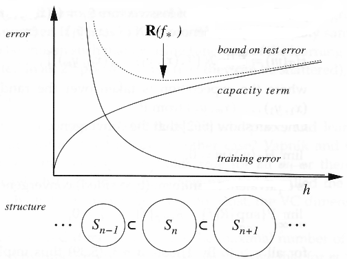
Notice that this result shows that we can obtain generalisaton error bounds for functions chosen from any of the hypothesis classes Hi. This is in contrast to Theorem 4.1, in which we needed to fix the class Hi in advance. This approach to trading off empirical error with hypothesis space complexity is known as Structural Risk Minimization (SRM). It is important to note that in order to apply SRM (using Theorem 4.1) we must define the hierarchy of hypothesis spaces before the data is observed. It is tempting to apply this result to support vector machines, since the following result shows that the VC dimension of large margin hyperplanes need not depend on the dimension of the feature space.
[…]
The bound suggests that maximising the margin performs SRM over the hypothesis spaces defined by a sequence of increasing margins, where we would define Hγ to be the space
Hγ = {f|f has margin at least γ on X0}.
The problem with this approach is that it violates one of the assumptions made in proving the SRM theorems, namely that the sequence of hypothesis spaces must be chosen before the data arrives. This is not possible, since a particular hyperplane can only be assigned to hypothesis space Hγ once we are able to measure its margin on the training data.
We will present a method for overcoming this problem which amounts to allowing the choice of the hierarchy of spaces to be dependent on the data (Shawe-Taylor et al., 1998). This analysis has been called data-dependent SMR for this reason. Intuitively, we may consider that the data is first used to decide which hierarchy to use, and then subsequently to choose the best hypothesis using the inherited measure of quality. For the example of large margins the hierarchies are those determined by the margins of hypotheses to the set of training points, and the inherited quality measure is the observed margin. The approach relies on a generalization of the VC dimension for real valued functions which is known as the fat-shattering dimension.”
Bartlett and Shawe-Taylor (1999), page 45-47
(3)
![]()
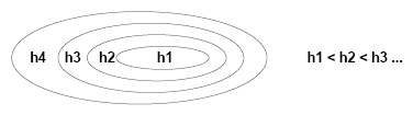
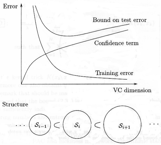
Figure 4. Nested subsets of functions, ordered by VC dimension.
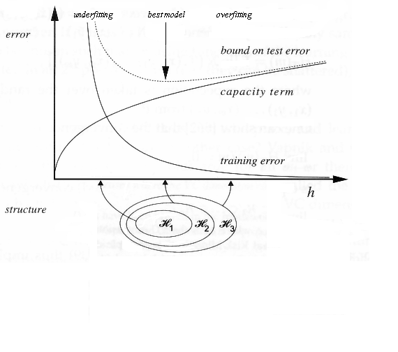
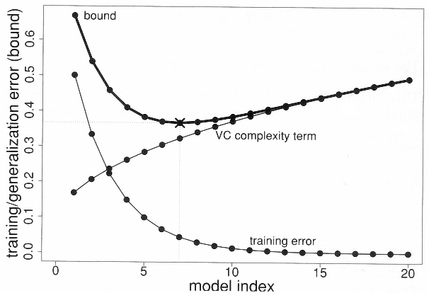
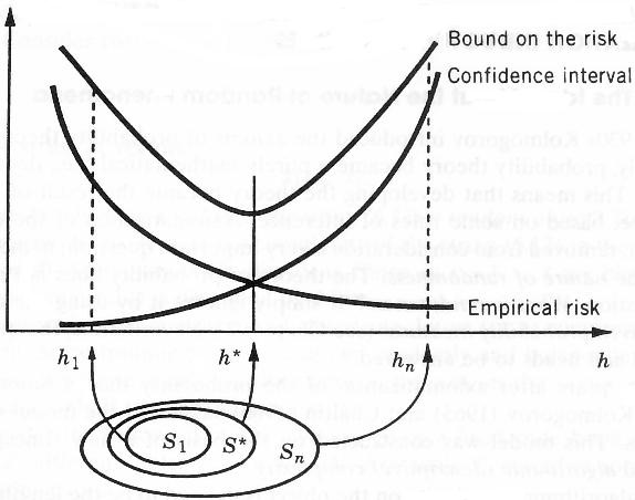
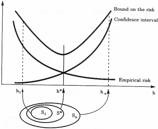
“We can now summarize the principle of structural risk minimization (SRM) (Vapnik, 1979). Note that the VC confidence term in Eq. (3) depends on the chosen class of functions, whereas the empirical risk and actual risk depend on the one particular function chosen by the training procedure. We would like to find that subset of the chosen set of functions, such that the risk bound for that subset is minimized. Clearly we cannot arrange things so that the VC dimension h varies smoothly, since it is an integer. Instead, introduce a “structure” by dividing the entire class of functions into nested subsets (Figure 4). For each subset, we must be able either to compute h, or to get a bound on h itself. SRM then consists of finding that subset of functions which minimizes the bound on the actual risk. This can be done by simply training a series of machines, one for each subset, where for a given subset the goal of training is simply to minimize the empirical risk. One then takes that trained machine in the series whose sum of empirical risk and VC confidence is minimal.”
[page 31] “…the argument does not constitute a rigorous demonstration of structural risk minimization for SVMs. The original argument for structural risk minimization for SVMs is known to be flawed, since the structure there is determined by the data (see (Vapnik, 1995), Section 5.11). I believe that there is a further subtle problem with the original argument. The structure is defined so that no training points are members of the margin set. However, one must still specify how test points that fall into the margin are to be labeled. If one simply assigns the same, fixed class to them (say +1), then the VC dimension will be higher21 than the bound derived in Theorem 6. However, the same is true if one labels them all as errors (see the Appendix). If one labels them all as “correct”, one arrives at gap tolerant classifiers.”
Burgess (1998)
Structural Risk Minimization (SRM) Under SRM, approximating functions of a learning machine are ordered according to their complexity, forming a nested structure:
[…]
For example, in the class of polynomial approximating functions, the elements of a structure are polynomials of a given degree. Condition (2.54) is satisfied, since polynomials of degree m are a subset of polynomials of degree (m + 1). The goal of learning is to choose an optimal element of a structure (i.e., polynomial degree) and estimate its coefficients from a given training sample. For approximating functions linear in parameters such as polynomials, the complexity is given by the number of free parameters. For functions nonlinear in parameters, the complexity is defined as VC-dimension (see Chapter 4). The optimal choice of model complexity provides the minimum of the expected risk. Statistical learning theory (Vapnik, 1995) provides analytic?? upper-bound estimates for expected risk. These estimates are used for model selection, namely choosing an optimal element of a structure under the SRM inductive principle.”
Cherkassky and Mulier (1998), page 45
![]()
“The inductive principle called structural risk minimization (SRM) provides a formal mechanism for choosing an optimal model complexity for a finite sample. SRM has been originally proposed and applied for classification (Vapnik and Chervonekis, 1974); however, it is applicable to any learning problem where the risk functional (4.1) has to be minimized. Under SRM the set […]
According to SRM, solving a learning problem with finite data requires a priori specification of a structure on a set of approximating (or loss) function. Then for a given data set, optimal model estimation amounts to two steps:
- Selecting an element of a structure (having optimal complexity).
- Estimating the model from this element.
Note that step (1) roughly corresponds to model order selection, whereas step (2) corresponds to parameter estimation in statistical methods. However, unlike statistical methods, SRM provides accurate analytical estimates for model selection based on generalization bounds presented in Section 4.3.
[…]
The SRM provides quantitative characterization of the trade-off between the complexity of approximating functions and the quality of fitting the training data. As the complexity (i.e., subset index k increases, the minimum of the empirical risk decreases (i.e., the quality of fitting the data improves), but the second additive term (the confidence interval) in (4.22) increases; see Fig 4.9. Similarly, for regression problems described by (4.29), with increased complexity the numerator (empirical risk) decreases, but the denominator becomes small (close to zero). The SRM chooses an optimal element of the structure that yields the minimal guaranteed bound on the true risk.
The SRM principle does not specify a particular structure. However, successful application of SRM in practice can depend on a chosen structure. […]
[…]
To implement the SRM approach using one of the above structures, in practice it is necessary to be able to (1) calculate or estimate VC-dimension of any element Sk of the structure and (2) minimize the empirical risk for any element Sk. This can be easily done for functions that are linear in parameters. However, for most practical methods using nonlinear approximating functions (e.g., neural networks) finding VC-dimension analytically is difficult, as is the nonlinear optimization problem of minimizing the empirical risk. There are various heuristic optimization procedures that are often used to implement SRM implicitly. Examples of such heuristics include early stopping rules and weight initialization (setting initial parameter values close to zero) which are often used in neural networks. Hence rigorous (analytic) application of the SRM principle can be difficult or impossible with nonlinear methods. This does not, however, imply that the statistical learning theory is impractical. In the next section we present an example of rigorous application of the SRM in the linear case. […]
Finally we emphasize that SRM does not specify the particular choice of approximating functions (polynomials, feedforward nets with sigmoid units, radial basis functions, etc.). Such a choice is outside the scope of SLT, and it should reflect a priori knowledge or subjective bias of a human modeler.”
Cherkassky and Mulier (1998), page 114-115
“The bound of Theorem 4.6 can be used to choose the hypothesis hi for which the bound is minimal, that is the reduction in the number of errors (first term) outweighs the increase in capacity (second term). This induction strategy is known as structural risk minimization.”
Cristianinin and Shawe-Taylor (2000)
“The idea of SRM is to define a nested sequence of hypothesis spaces F1 ⊂ F2 ⊂ … ⊂ Fn(m) with n(m) a non-decreasing integer function of m, where each hypothesis space Fi has VC-dimension finite and larger than that of all previous sets, i.e., if hi is the VC-dimension of space Fi, then h1 ≤ h2 ≤ … ≤ hn(m). For example Fi could be the set of polynomials of degree i, or a set of splines with i nodes, or some more complicated nonlinear parameterization […]”
Evgeniou, Pontil and Poggio (2000), page 178
“Vapnik’s structural risk minimization approach fits a nested sequence of models of increasing VC dimensions h1 < h2 < …, and then chooses the model with the smallest value of the upper bound.
We note that upper bounds like the ones in (7.41) are often very loose, but that doesn’t rule them out as good criteria for model selection, where the relative (not absolute) size of the test error is important. The main drawback of this approach is the difficulty in calculating the VC dimension of a class of functions. Often only a crude upper bound for VC dimension is obtainable, and this may not be adequate. An example in which the structural risk minimization program can be successfully carried out is the support vector classifier, discussed in Section 12.2.”
Hastie, Tibshirani and Friedman (2001), page 212
“We shall see that there exist several measures of “complexity” of hypothesis spaces, the VC dimension being the most prominent thereof. V. Vapnik suggested a learning principle which he called structural risk minimization (SRM). The idea behind SRM is to, a-priori, define a structuring of the hypothesis space F into nested subsets F0 ⊂ F1 ⊂ … ⊆ F of increasing complexity. Then, in each of the hypothesis spaces Fi empirical risk minimization is performed. Based on results from statistical learning theory, an SRM algorithm returns the classifier with the smallest guaranteed risk8 [This is a misnomer as it refers to the value of an upper bound at a fixed confidence level and can in no way be guaranteed.]. This can be related to the algorithm (2.14), if Ω[f] is the complexity value of f given by the used bound for the guaranteed risk.” page 29
[…]
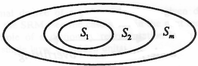
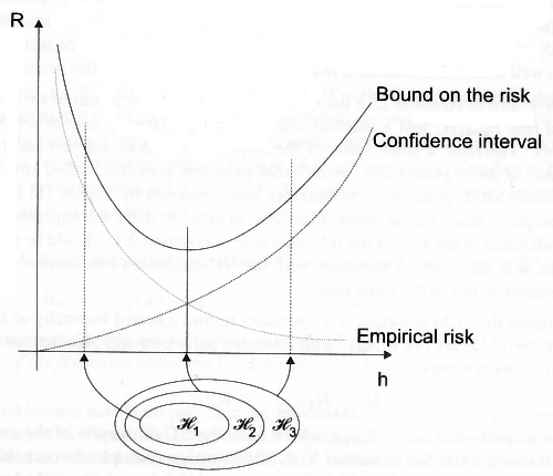
One possible method of overcoming this problem is to use the principle of structural risk minimization (SRM). By a structure we mean a set S = {H1, …, Hs of s hypothesis spaces. It is often assumed that […]. Clearly we cannot directly apply Theorems 4.7 because they assume a fixed hypothesis space. Further, we might have some prior hope that the minimizer of the expected risk is within equivalence class Hi which we express by a probability distribution […]. In order to get a theoretically justified result we make use of the following lemma which is the basis of multiple testing5.[…] […] Note that the SRM principle is a curious one: In order to have an algorithm it is necessary to have a good theoretical bound on the generalization error of the empirical risk minimization method. Another view of the structural risk minimization principle is that it is an attempt to solve the model selection problem. In place of the ultimate quantity to be minimized—the expected risk of the learned function […]—a (probabilistic) bound on the latter is used, automatically giving a performance guarantee of the model selection principle itself.”
“Figure 4.4 Structural risk minimization in action. Here we used hypothesis spaces Hi such that […]. This implies that the training errors of the empirical risk minimizers can only be decreasing which leads to the typical situation depicted. Note that lines are used for visualization purposes because we consider only a finite set S of hypothesis spaces.” page 134
Using structural risk minimization we are able to make the complexity, as measured by the VC dimension of the hypothesis space, a variable of a model selection algorithm while still having guarantees for the expected risks. Nonetheless, we recall that the decomposition of the hypothesis space must be done independently of the observed training sample z. This rule certainly limits the applicability of structural risk minimization to an a-priori complexity penalization strategy. The resulting bounds effectively ignore the sample z ∈ Zm except with regard to the training error Remp[A(z), z]. A prominent example of the misuse of structural risk minimization was the first generalization error bounds for the support vector machine algorithm. It has become commonly accepted that the success of support vector machines can be explained through the structuring of the hypothesis space H of linear classifiers in terms of the geometrical margin γz(w) of a linear classifier having normal vector w (see Definition 2.30). Obviously, however, the margin itself is a quantity that strongly depends on the sample z and thus a rigorous application of structural risk minimization is impossible! Nethertheless, we shall see in the following section that the margin is, in fact, a quantity which allows an algorithm to control its generalization error.
In order to overcome this limitation we will introduce the luckiness framework.”
Herbrich (2002)
“The idea of structural risk minimization is to find a hypothesis h from a hypothesis space H for which one can guarantee the lowest probability of error Err(h) for a given training sample S […]
of n examples. The following upper bound connects the true error of a hypothesis h with the error Errtrain(h) of h on the training set and the complexity of h [Vapnik, 1998] (see also Section 1.1).
[…]
The bound holds with a probability of at least 1 – η. d denotes the VC-dimemsion [Vapnik, 1998], which is a property of the hypothesis space H and indicates its expressiveness. Equation (3.2) reflects the well-known trade-off between the complexity of the hypothesis space and the training error. A simple hypothesis space (small VC-dimension) will probably not contain good approximating functions and will lead to a high training (and true) error. On the other hand a too rich hypothesis space (large VC-dimension) will lead to a small training error, but the second term in the right-hand side of (3.2) will be large. This reflects the fact that for a hypothesis space with a high VC-dimension the hypothesis with low training error may just happen to fit the training data without accurately predicting new examples. This situation is commonly called “overfitting”. It is crucial to pick the hypothesis space with the “right” complexity.
In Structural Risk Minimization this is done by defining a nested structure of hypothesis spaces Hi, so that their respective VC-dimension di increases.
[…]
This structure has to be defined a priori, i.e. before analyzing the training data. The goal is to find the index i* for which (3.2) is minimum.
[…]
[page 38] How do support vector machines implement structural risk minimization? Vapnik showed that there is a connection between the margin and the VC-dimension.”
Joachims (2002)
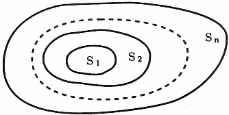
Structural risk minimization is a novel inductive principle for learning from finite training data sets. It is very useful when dealing with small samples. The basic idea of SRM is to choose, from a large number of candidate models (learning machines), a model of the right complexity to describe training data pairs. As previously stated, this can be done by restricting the hypothesis space H of approximating functions and simultaneously controlling their flexibility (complexity). Thus, learning machines will be those parameterized models that, by increasing the number of parameters (called weights w here), form a nested structure in the following sense:
H1 ⊂ H2 ⊂ H3 ⊂ … ⊂ Hn – 1 ⊂ Hn ⊂ … ⊂ H. (2.35)
In such a nested set of functions, every function always contains a previous, less complex, function (for a sketch of this nested set idea, see fig. 2.6). Typically, Hn may be a set of polynomials in one variable of degree n; a fuzzy logic (FL) model having n rules; multilayer perceptrons; or an RBF network having n hidden layer neurons. The definition of nested sets (2.35) is satisfied for all these models because, for example, an NN with n neurons is a subset of an NN with n + 1 neurons, an FL model comprising n rules is a subset of an FL model comprising n + 1 rules, and so on. The goal of learning is one of subset selection, which matches training data complexity with approximating model capacity. In other words, a learning algorithm chooses an optimal polynomial degree or an optimal number of hidden layer neurons or an optimal number of FL model rules.
[…]
Now, almost all the basic ideas and tools needed in the statistical learning theory and in structural risk minimization have been introduced. At this point, it should be clearer how an SRM works—it uses the VC dimension as a controlling parameter (through a determination of confidence interval) for minimizing the generalization bound R(wn) given in (2.36). However, some information about how an SVM implements the SRM principle is still missing. One needs to show that SVM learning actually minimizes both the VC dimension (confidence interval, estimation error) and the approximation error (empirical risk) at the same time. This proof is given later.
Kecman (2001)
Before applications of OCSH for both overlapping classes and classes having nonlinear decision boundaries are presented, it must be shown that SV-based linear classifiers actually implement the SRM principle. In other words, we must prove that SV machine training actually minimizes both the VC dimension and a generalization error at the same time. In section 2.2, it was stated that the VC dimension of the oriented hyperplane indicator function, in an n-dimensional space of features, is equal to n + 1 (i.e., h = n + 1). It was also demonstrated that the RBF neural network (or the SVM having RBF kernels) can shatter infinitely many points (its VC dimension can be infinitely large, h = ∞). Thus, an SVM could have a very high VC dimension. At the same time, in order to keep the generalization error (bound on the test error) low, the confidence interval (the second term on the right-hand side of (2.36a)) was minimized by imposing a structure on the set of approximating functions (see fig. 2.13).
[…]
Kecman (2001), page 161
“Vapnik’s (1982) structural risk minimization is a similar idea, using a bound on test-set risk based on the work of Section 2.8 and discussed further there.”
Ripley (1996), page 62
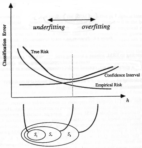
“The empirical risk minimization principle described above turns out to be not optimal. It does not guarantee a small actual risk R([alpha]) also named generalization error (i.e. a small error on the training set S does not imply a small error on an independent but indentically distributed test set), if the number of training examples is limited [100, 116]. This fact can be seen in figure 2.4. If the system complexity h is increased the empirical risk can be reduced aribitrarily. At the same time the actual risk will decrease up to a certain point and than (sic) increase again. This behavior is known as over-fitting from neural network theory, and can be interpreted as a memorization of the training patterns instead of learning the underlying functional dependencies. When using Multilayer Perceptrons or Radial Basis Functions network this is equivalent to the problem of finding the appropriate number of hidden neurons (this is called model selection), which is known to be a difficult problem. Many approaches have been developed to overcome this problem, e.g. neural network pruning (see chapter 3 section 3.3 below for some new methods), neural network growing [129, 130] and cross-validation techniques for the selection process (see section 2.4). An approach well founded in statistical learning theory is described in this section.
[…]
The implementation of the SRM principle can be difficult because of two reasons: At first it is often difficult to find the VC-dimension for a hypothesis space Hn, since not for all models and machines it is known how to calculate this. And the second point is that even if it is possible to compute hn (or a bound on it) of Hn it is not trivial to solve the optimization problem that is given by 2.15. In most cases this has to be done by simply training a series of machines, one for each subset, and the (sic) choosing that Hn that gives the lowest risk bound.
To summarize the structural risk minimization principle is clearly well founded mathematically, but it can be difficult to realize. The support vector machine achieves the goal of the SRM principle, minimizing a bound on the VC-dimension and the training error concurrently, by a completely automatic optimization procedure.”
Rychetsky (2001)
“The function class is decomposed into a nested sequence of subsets of increasing size (and thus, of increasing capacity). The SRM principle picks a function f* which has small training error, and comes from an element of the structure that has low capacity h, thus minimizing a risk bound of type (5.36).”
Schölkopf and Smola (2002), page 139
“In order to apply the VC bound to SVM classifiers, Vapnik employs the concept of so-called structural risk minimization. One considers a structure
[…]
which consists of nested sets of functions of increasing complexity. This is illustrated in Fig.2.10 [206]. The concept is quite similar to previously discussed complexity criteria and bias-variance trade-off curves. In this case of VC theory one may consider sets of functions with increasing VC dimension. The larger this VC dimension the smaller the training set error can become (empirical risk) but the confidence term (second term in (2.34)) will grow. The minimum of the sum of these two terms is then a good compromise solution as the trade-off between these two curves.
For SVM classifiers one can find an upper bound on the VC dimension as follows. Vapnik has shown that hyperplanes satisfying ||w||2 < a have a VC-dimension h which is upper bounded by
h ≤ min([r2a2], n) + 1 (2.36) where [⋅] denotes the integer part and r is the radius of the smallest ball containing the points φ(x1), …, φ(xN) in the high dimensional feature space (Fig. 2.11).”
Suykens, et al. (2002), page 48
Vapnik and Chernovenkis suggest choosing for each N the function [?] according to the structural risk minimization principle (SRM). This consists of the following two steps. First we select the classifier [?] from every class [?] that minimizes the corresponding empirical error over the class of functions. Then, from all these classifiers, we choose the one that minimizes the upper bound in (5.36), over all i. More precisely, form the so-called guaranteed error bound, […]
[…]
From this point of view, the structural risk minimization principle belongs to a more general class of approaches that try to estimate the order of a system, by considering simultaneously the model complexity and a performance index. […]
The SRM procedure provides a theoretical guideline for constructing a classifier that converges asymptotically to the optimal Bayesian one. However, the bound in (5.36) which is exploited in order to reach this limit, must not be misinterpreted. For any bound to be useful in practice, one needs an extra piece of information. Is this bound loose or tight? In general, until now, there has been no result that provides this information. We can construct classifiers whose VC dimension is large, yet their performance can be good.
[…]
Thus, we can conclude that, the design of an SVM classifier senses the spirit of the SRM principle Theodoridis and Koutroumbas (2003)
“For a given set of observations z1, …, zl the SRM method chooses the element Sk of the structure for which the smallest bound on the risk (the smallest guaranteed risk) is achieved.
Therefore the idea of the structural risk minimization induction principle is the following:
To provide the given set of functions with an admissible structure and then to find the function that minimizes guaranteed risk (6.8) (or (6.9)) over given elements of the structure.
To stress the importance of choosing the element of the structure that possesses an appropriate capacity, we call this principle the principle of structural rism minimization. It describes a general model of capacity control. To find the guaranteed risk, one has to use bounds on the actual risk. As shown in previous chapters, all of them have to contain information about the capacity of the element of the structure to which the chosen function belongs. In this chapter, we will use the bounds (6.8) or (6.9).
Section 6.3 shows that the SRM principle is always consistent and defines a bound on the rate of convergence. However, we must first describe the Minimum Description Length principle and point out its connection to the SRM principle for pattern recognition problem.”
Vapnik (1998)
“The following general principle, which is called the structural risk minimization (SRM) inductive principle, is intended to minimize the risk functional with respect to both terms, the empirical risk, and the confidence interval (Vapnik and Chervonenkis, 1974).
[…]
The SRM principle defines a trade-off between the quality of the approximation of the given data and the complexity of the approximating function. As the subset index n increases, the minima of the empirical risks decrease. However, the term responsible for the confidence interval (the second summand in inequality (4.1) or the multiplier in inequality (4.2) (Fig. 4.2)) increases. The SRM principle takes both factors into account by choosing the subset Sn for which minimizing the empirical risk yields the best bound on the actual risk.”
Vapnik (2000)
“An example of an extension of the VC framework (which actually came to prominence about the same time as the original work) is “structural risk minimumization.” Loosely speaking, in structural risk minimization, one has several generalizers51 forming a nested hypothesis class structure, H~1 ⊂ H~2 ⊂ …. One parses the set of generalizers to find the generalizer that by itself (i.e., according to the VC dimension of the associated H~i) has the best confidence interval. The nesting means that to an often good approximation we can assign that “best confidence interval” to our generalizer’s guess, despite our having parsed a set of generalizers to arrive at that guess. Without nesting, generically one would have to treat the entire parsing algorithm along with the underlying generalizers as simply a new learning algorithm, with VC dimension determined by the union of the H~i. In such a situation, one would not be able to exploit differences in the VC dimensions of the constituent H~i.”
Wolpert (1995)
Bibliography
- AZIMI-SADJADI, M.R. and S.A. ZEKAVAT, 2000. Cloud classification using support vector machines. Geoscience and Remote Sensing Symposium, 2000. Proceedings. …. [Cited by 22] (2.68/year)
- BAHLMANN, C., B. HAASDONK and H. BURKHARDT, 2002. On-line Handwriting Recognition with Support Vector Machines?A Kernel Approach. Proc. of the 8th IWFHR. [Cited by 103] (16.57/year)
- BARTLETT, P.L., O. BOUSQUET and S. MENDELSON, 2002. Localized Rademacher Complexities. LECTURE NOTES IN COMPUTER SCIENCE. [Cited by 88] (14.15/year)
- BARTLETT, P.L., S. MENDELSON and P.M. LONG, 2003. Rademacher and Gaussian Complexities: Risk Bounds and Structural Results. Journal of Machine Learning Research. [Cited by 157] (30.09/year)
- BEN-YACOUB, S., Y. ABDELJAOUED and E. MAYORAZ, 1999. Fusion of face and speech data for person identity verification. IEEE Transactions on Neural Networks. [Cited by 155] (16.82/year)
- BENNETT, K. and A. DEMIRIZ, 1999. Semi-Supervised Support Vector Machines. ADVANCES IN NEURAL INFORMATION PROCESSING SYSTEMS. [Cited by 213] (23.11/year)
- BENNETT, K.P. and J.A. BLUE, 1998. A support vector machine approach to decision trees. Neural Networks Proceedings, 1998. IEEE World Congress on …. [Cited by 59] (5.77/year)
- BLANZ, V., et al., 1996. Comparison of view {based object recognition algorithms using realistic 3D models. Artificial Neural Networks: ICANN 96: 1996 International …. [Cited by 119] (9.74/year)
- BURBIDGE, R., et al., 2001. Drug design by machine learning: support vector machines for pharmaceutical data analysis. Computers and Chemistry. [Cited by 197] (27.30/year)
- BURGES, C.J.C., 1998. A Tutorial on Support Vector Machines for Pattern Recognition. Data Mining and Knowledge Discovery. [Cited by 4678] (457.86/year)
- CAMPS-VALLS, G. and L. BRUZZONE, 2005. Kernel-based methods for hyperspectral image classification. Geoscience and Remote Sensing, IEEE Transactions on. [Cited by 51] (15.85/year)
- CHEN, S., A.K. SAMINGAN and L. HANZO, 2001. Support vector machine multiuser receiver for DS-CDMA signals inmultipath channels. Neural Networks, IEEE Transactions on. [Cited by 92] (12.75/year)
- CLARKSON, P. and P.J. MORENO, 1999. On the use of support vector machines for phonetic classification. Acoustics, Speech, and Signal Processing, 1999. ICASSP’99. …. [Cited by 84] (9.11/year)
- CORTES, C. and V. VAPNIK, 1995. Support-vector networks. Machine Learning. [Cited by 3688] (279.03/year)
- CRISTIANINI, N., C. CAMPBELL and J. SHAWE-TAYLOR, 1999. Dynamically Adapting Kernels in Support Vector Machines. ADVANCES IN NEURAL INFORMATION PROCESSING SYSTEMS. [Cited by 94] (10.20/year)
- D?NIZ, O., M. CASTRILL?N and M. HERN?NDEZ, 2003. Face recognition using independent component analysis and support vector machines. Pattern Recognition Letters. [Cited by 64] (12.27/year)
- DING, A.L., X.M. ZHAO and L.C. JIAO, 2002. Traffic flow time series prediction based on statistics learning theory. Intelligent Transportation Systems, 2002. Proceedings. The …. [Cited by 13] (2.09/year)
- DUAN, K., S.S. KEERTHI and A.N. POO, 2003. Evaluation of simple performance measures for tuning SVM hyperparameters. Neurocomputing. [Cited by 140] (26.83/year)
- EL-NAQA, I., et al., 2002. Support vector machine learning for detection of microcalcifications in mammograms. Biomedical Imaging, 2002. Proceedings. 2002 IEEE …. [Cited by 20] (3.22/year)
- EL-NAQA, I., et al., 2002. A Support Vector Machine Approach for Detection of Microcalcifications. IEEE TRANSACTIONS ON MEDICAL IMAGING. [Cited by 95] (15.28/year)
- EVGENIOU, T., et al., 2002. Regularization and statistical learning theory for data analysis. Computational Statistics and Data Analysis. [Cited by 20] (3.22/year)
- EVGENIOU, T., M. PONTIL and T. POGGIO, 2000. Statistical Learning Theory: A Primer. International Journal of Computer Vision. [Cited by 22] (2.68/year)
- EVGENIOU, T., M. PONTIL and T. POGGIO, 2000. Regularization Networks and Support Vector Machines. Advances in Computational Mathematics. [Cited by 494] (60.12/year)
- FAN, A. and M. PALANISWAMI, 2000. Selecting bankruptcy predictors using a support vector machineapproach. Neural Networks, 2000. IJCNN 2000, Proceedings of the IEEE- …. [Cited by 29] (3.53/year)
- GANAPATHIRAJU, A., et al., 2004. Applications of support vector machines to speech recognition. Signal Processing, IEEE Transactions on [see also Acoustics, …. [Cited by 43] (10.20/year)
- GANAPATHIRAJU, A., J. HAMAKER and J. PICONE, 1998. Support Vector Machines for Speech Recognition. Fifth International Conference on Spoken Language Processing. [Cited by 64] (6.26/year)
- GANAPATHIRAJU, A., J. HAMAKER and J. PICONE, 2000. Hybrid SVM/HMM Architectures for Speech Recognition. Sixth International Conference on Spoken Language Processing. [Cited by 42] (5.11/year)
- GAO, J.B., et al., 2002. A Probabilistic Framework for SVM Regression and Error Bar Estimation. Machine Learning. [Cited by 37] (5.95/year)
- GAO, J.B., C.J. HARRIS and S.R. GUNN, 2001. On a Class of Support Vector Kernels Based on Frames in Function Hilbert Spaces. Neural Computation. [Cited by 18] (2.49/year)
- GIROSI, F., 1998. An Equivalence Between Sparse Approximation and Support Vector Machines. Neural Computation. [Cited by 334] (32.69/year)
- GUERMEUR, Y., et al., 2000. A new multi-class SVM based on a uniform convergence result. Neural Networks, 2000. IJCNN 2000, Proceedings of the IEEE- …. [Cited by 42] (5.11/year)
- GUYON, I., et al., 1992. Structural risk minimization for character recognition. Advances in Neural Information Processing Systems. [Cited by 73] (4.50/year)
- HERBRICH, R., 2002. Learning kernel classifiers. mitpress.mit.edu. [Cited by 103] (16.57/year)
- HERBRICH, R., et al., 1998. Learning preference relations for information retrieval. ICML-98 Workshop: Text Categorization and Machine Learning. [Cited by 33] (3.23/year)
- HUANG, C., L.S. DAVIS and J.R.G. TOWNSHEND, 2002. An assessment of support vector machines for land cover classification. International Journal of Remote Sensing. [Cited by 114] (18.34/year)
- JOACHIMS, T., 1997. Text Categorization with Support Vector Machines: Learning with Many Relevant Features. Springer. [Cited by 2729] (243.29/year)
- JOACHIMS, T., 1999. Transductive Inference for Text Classification using Support Vector Machines. MACHINE LEARNING-INTERNATIONAL WORKSHOP THEN CONFERENCE-. [Cited by 730] (79.20/year)
- JOACHIMS, T., 2003. Transductive Learning via Spectral Graph Partitioning. MACHINE LEARNING-INTERNATIONAL WORKSHOP THEN CONFERENCE-. [Cited by 168] (32.20/year)
- KALOUSIS, A., J. GAMA and M. HILARIO, 2004. On Data and Algorithms: Understanding Inductive Performance. Machine Learning. [Cited by 11] (2.61/year)
- KARA?ALI, B., R. RAMANATH and W.E. SNYDER, 2004. A comparative analysis of structural risk minimization by support vector machines and nearest …. Pattern Recognition Letters. [Cited by 11] (2.61/year)
- KARACALI, B. and H. KRIM, 2003. Fast minimization of structural risk by nearest neighbor rule. Neural Networks, IEEE Transactions on. [Cited by 20] (3.83/year)
- KHARROUBI, J., D. PETROVSKA-DELACRETAZ and G. CHOLLET, 2001. Combining GMM’s with Suport Vector Machines for Text-independent Speaker Verification. Seventh European Conference on Speech Communication and …. [Cited by 16] (2.22/year)
- KIM, D., 2004. Structural Risk Minimization on Decision Trees Using an Evolutionary Multiobjective Optimization. LECTURE NOTES IN COMPUTER SCIENCE. [Cited by 8] (1.90/year)
- KIM, H., et al., 2002. Pattern Classification Using Support Vector Machine Ensemble. INTERNATIONAL CONFERENCE ON PATTERN RECOGNITION. [Cited by 38] (6.11/year)
- KIM, H.C., et al., 2003. Constructing support vector machine ensemble. Pattern Recognition. [Cited by 71] (13.61/year)
- KIM, K.I., et al., 2002. Support Vector Machines for Texture Classification. IEEE TRANSACTIONS ON PATTERN ANALYSIS AND MACHINE …. [Cited by 117] (18.82/year)
- KIM, K.J., 2003. Financial time series forecasting using support vector machines. Neurocomputing. [Cited by 92] (17.63/year)
- KOHLER, M., A. KRZYZAK and D. SCH?FER, 2002. Application of structural risk minimization to multivariate smoothing spline regression estimates. Bernoulli. [Cited by 4] (0.64/year)
- KOLTCHINSKII, V., 2001. Rademacher penalties and structural risk minimization. Information Theory, IEEE Transactions on. [Cited by 73] (10.11/year)
- KWOK, J.T.Y., 1998. Support Vector Mixture for Classification and Regression Problems. INTERNATIONAL CONFERENCE ON PATTERN RECOGNITION. [Cited by 53] (5.19/year)
- KWOK, J.T.Y., 1999. Moderating the outputs of support vector machine classifiers. Neural Networks, IEEE Transactions on. [Cited by 90] (9.76/year)
- LEE, J.W., et al., 2005. An extensive comparison of recent classification tools applied to microarray data. Computational Statistics and Data Analysis. [Cited by 51] (15.85/year)
- LI, Y., S. GONG and H. LIDDELL, 2000. Support vector regression and classification based multi-view face detection and recognition. IEEE International Conference on Automatic Face & Gesture …. [Cited by 104] (12.66/year)
- LIONG, S.Y. and C. SIVAPRAGASAM, 2002. FLOOD STAGE FORECASTING WITH SUPPORT VECTOR MACHINES 1. Journal of the American Water Resources Association. [Cited by 30] (4.83/year)
- LIU, H.P.H.Y.H., 2002. Fuzzy Support Vector Machines for Pattern Recognition and Data Mining. International Journal of Fuzzy Systems. [Cited by 97] (15.60/year)
- LOZANO, F., 2000. Model selection using Rademacher penalization. Proceedings of the Second ICSC Symposia on Neural …. [Cited by 12] (1.46/year)
- LUGOSI, G. and K. ZEGER, 1996. Concept learning using complexity regularization. Information Theory, IEEE Transactions on. [Cited by 40] (3.27/year)
- MA, C., M.A. RANDOLPH and J. DRISH, 2001. A support vector machines-based rejection technique for speechrecognition. Acoustics, Speech, and Signal Processing, 2001. Proceedings. …. [Cited by 30] (4.16/year)
- MIKA, S., G. RATSCH and K.R. MULLER, 2001. A Mathematical Programming Approach to the Kernel Fisher Algorithm. ADVANCES IN NEURAL INFORMATION PROCESSING SYSTEMS. [Cited by 102] (14.13/year)
- MORIK, K., P. BROCKHAUSEN and T. JOACHIMS, 1999. Combining statistical learning with a knowledge-based approach-A case study in intensive care …. MACHINE LEARNING-INTERNATIONAL WORKSHOP THEN CONFERENCE-. [Cited by 127] (13.78/year)
- MUKHERJEE, S., E. OSUNA and F. GIROSI, 1997. Nonlinear prediction of chaotic time series using support vectormachines. Neural Networks for Signal Processing [1997] VII. …. [Cited by 258] (23.00/year)
- NIYOGI, P., C. BURGES and P. RAMESH, 1999. Distinctive feature detection using support vector machines. Acoustics, Speech, and Signal Processing, 1999. ICASSP’99. …. [Cited by 50] (5.42/year)
- OSUNA, E. and F. GIROSI, 1999. Reducing the run-time complexity of support vector machines. Advances in Kernel Methods: Support Vector Learning, MIT …. [Cited by 114] (12.37/year)
- OSUNA, E., R. FREUND and F. GIROSI, An improved training algorithm for support vector machines. ieeexplore.ieee.org. [Cited by 614] (?/year)
- OSUNA, E., R. FREUND and F. GIROSI, 1997. Support Vector Machines: Training and Applications. [Cited by 395] (35.21/year)
- PAI, P.F. and W.C. HONG, 2005. Forecasting regional electricity load based on recurrent support vector machines with genetic …. Electric Power Systems Research. [Cited by 37] (11.50/year)
- PHILLIPS, P.J. and N.A.T.I.O.N.A.L. INSTITUTE, 1998. Support Vector Machines Applied to Face Recognition. [Cited by 142] (13.90/year)
- RUPING, S. and K. MORIK, 2003. Support vector machines and learning about time. Acoustics, Speech, and Signal Processing, 2003. Proceedings. …. [Cited by 12] (2.30/year)
- SAMANTA, B., K.R. AL-BALUSHI and S.A. AL-ARAIMI, 2003. Artificial neural networks and support vector machines with genetic algorithm for bearing fault …. Engineering Applications of Artificial Intelligence. [Cited by 44] (8.43/year)
- SAN, L. and M. GE, 2004. An effective learning approach for nonlinear system modeling. Intelligent Control, 2004. Proceedings of the 2004 IEEE …. [Cited by 6] (1.42/year)
- SCHOHN, G. and D. COHN, 2000. Less is More: Active Learning with Support Vector Machines. MACHINE LEARNING-INTERNATIONAL WORKSHOP THEN CONFERENCE-. [Cited by 204] (24.83/year)
- SCHOLKOPF, B., et al., 1997. Comparing support vector machines with Gaussian kernels to radial basis function classifiers. IEEE Transactions on Signal Processing. [Cited by 426] (37.98/year)
- SCOTT, C. and R. NOWAK, 2003. Dyadic Classification Trees via Structural Risk Minimization. Advances in Neural Information Processing Systems 15: …. [Cited by 17] (3.26/year)
- SHAWE-TAYLOR, J. and N. CRISTIANINI, 1998. Data-Dependent Structural Risk Minimization for Perceptron Decision Trees. ADVANCES IN NEURAL INFORMATION PROCESSING SYSTEMS. [Cited by 19] (1.86/year)
- SHAWE-TAYLOR, J., et al., Structural Risk Minimization over Data-Dependent Hierarchies, Neuro-COLT Technical Report NC-TR-96- …. [Cited by 4] (?/year)
- SHAWE-TAYLOR, J., et al., 1998. Structural risk minimization over data-dependent hierarchies. Information Theory, IEEE Transactions on. [Cited by 298] (29.17/year)
- SHAWE-TAYLOR, J., et al., lip;. Structural Risk Minimization over Data-Dependent Hierarchies, to appear in IEEE Trans. on Inf. …. and NeuroCOLT Technical Report NC-TR-96-053, 1996.(ftp://ftp. &h. [Cited by 5] (?/year)
- SHAWE-TAYLOR, J., P.L. BARTLETT and R.C. WILLIAMSON, Anthony, & M.(1998). Structural risk minimization over data-dependent hierarchies. IEEE Transactions on Information Theory. [Cited by 3] (?/year)
- SUGIYAMA, M. and H. OGAWA, 2001. Subspace Information Criterion for Model Selection. Neural Computation. [Cited by 62] (8.59/year)
- SUN, Z., G. BEBIS and R. MILLER, 2002. On-road vehicle detection using gabor filters and support vector machines. International Conference on Digital Signal Processing. [Cited by 45] (7.24/year)
- SUYKENS, J.A.K. and J. VANDEWALLE, 1999. Training multilayer perceptron classifiers based on a modifiedsupport vector method. Neural Networks, IEEE Transactions on. [Cited by 21] (2.28/year)
- SUYKENS, J.A.K. and J. VANDEWALLE, 1999. Least Squares Support Vector Machine Classifiers. Neural Processing Letters. [Cited by 829] (89.94/year)
- SUYKENS, J.A.K., 2001. Nonlinear modelling and support vector machines. Instrumentation and Measurement Technology Conference, 2001. …. [Cited by 118] (16.35/year)
- SUYKENS, J.A.K., 2002. Least Squares Support Vector Machines. books.google.com. [Cited by 644] (103.58/year)
- SUYKENS, J.A.K., et al., 1999. Least squares support vector machine classifiers: a large scale algorithm. Proceedings of the European Conference on Circuit Theory and …. [Cited by 82] (8.90/year)
- SYED, N.A., H. LIU and K.K. SUNG, 1999. A study of support vectors on model independent example selection. Proceedings of the fifth ACM SIGKDD international conference …. [Cited by 25] (2.71/year)
- SYED, N.A., H. LIU and K.K. SUNG, 1999. Handling concept drifts in incremental learning with support vector machines. Proceedings of the fifth ACM SIGKDD international conference …. [Cited by 184] (19.96/year)
- TAPIA, E. and R. ROJAS, 2003. Recognition of on-line handwritten mathematical formulas in the E-chalk system. Document Analysis and Recognition, 2003. Proceedings. …. [Cited by 21] (4.03/year)
- TAY, F.E.H. and L. CAO, 2001. Application of support vector machines in ?nancial time series forecasting. Omega. [Cited by 178] (24.66/year)
- TAY, F.E.H. and L.J. CAO, 2002. Modi?ed support vector machines in ?nancial time series forecasting. Neurocomputing. [Cited by 115] (18.50/year)
- TAY, F.E.H., 2001. A comparative study of saliency analysis and genetic algorithm for feature selection in support …. Intelligent Data Analysis. [Cited by 19] (2.63/year)
- VAPNIK, V. and A. STERIN, 1977. On structural risk minimization or overall risk in a problem of pattern recognition. Automation and Remote Control. [Cited by 10] (0.32/year)
- VAPNIK, V. and L. BOTTOU, 1993. Local Algorithms for Pattern Recognition and Dependencies Estimation. Neural Computation. [Cited by 54] (3.55/year)
- VAPNIK, V.N., 1999. An overview of statistical learning theory. Neural Networks, IEEE Transactions on. [Cited by 833] (90.37/year)
- VERZI, S.J., et al., 2001. Rademacher penalization applied to fuzzy ARTMAP and boosted ARTMAP. Neural Networks, 2001. Proceedings. IJCNN’01. International …. [Cited by 20] (2.77/year)
- VIOLA, P. and M. JONES, 2002. Fast and Robust Classification using Asymmetric AdaBoost and a Detector Cascade. ADVANCES IN NEURAL INFORMATION PROCESSING SYSTEMS. [Cited by 116] (18.66/year)
- YANG, M.H., D. ROTH and N. AHUJA, 2000. Learning to Recognize 3D Objects with SNoW. LECTURE NOTES IN COMPUTER SCIENCE. [Cited by 31] (3.77/year)
- ZHANG, J., et al., log. Modified Logistic Regression: An Approximation to SVM and Its Applications in Large-Scale Text …. [Cited by 38] (?/year)
- ZHANG, J., X. DING and C. LIU, 2000. Multi-scale feature extraction and nested-subset classifier designfor high accuracy handwritten …. Pattern Recognition, 2000. Proceedings. 15th International …. [Cited by 19] (2.31/year)
- ZHAO, Q. and J.C. PRINCIPE, 2001. Support vector machines for SAR automatic target recognition. Aerospace and Electronic Systems, IEEE Transactions on. [Cited by 60] (8.31/year)
Leave a Reply
You must be logged in to post a comment.