Sellaholics.com – Find Top 10 Products in Every Category
VC Dimension
VC dimension (for Vapnik Chervonenkis dimension) (Vapnik and Chervonenkis (1968, 1971), Vapnik (1979)) measures the capacity of a hypothesis space. Capacity is a measure of complexity and measures the expressive power, richness or flexibility of a set of functions by assessing how wiggly its members can be.
Sewell (2006)
“Let us say we have a dataset containing N points. These N points can be labeled in 2N ways as positive and negative. Therefore, 2N different learning problems can be defined by N data points. If for any of these problems, we can find a hypothesis h ∈ H that separates the positive examples from the negative, then we say H shatters N points. That is, any learning problem definable by N examples can be learned with no error by a hypothesis drawn from H. The maximum number of points that can be shatttered by H is called the Vapnik-Chervonekis (VC) dimension of H, is denoted as VC(H), and measures the capacity of the hypothesis class H.
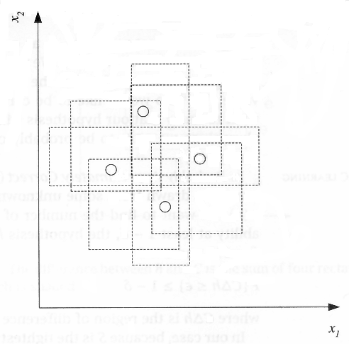
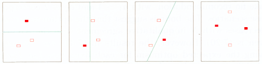
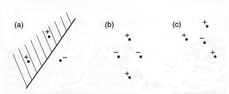
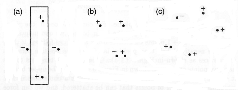
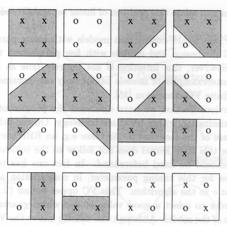
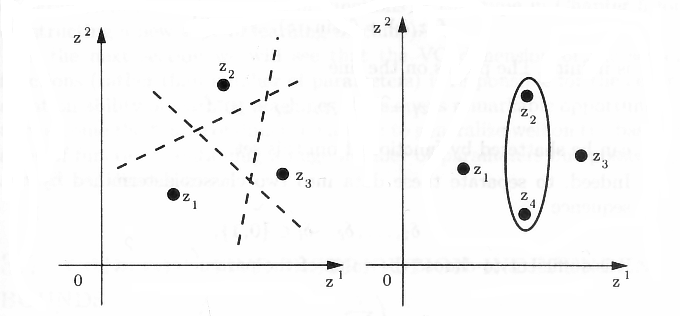
In figure 2.5, we see that an axis-aligned rectangle can shatter four points in two dimensions. Then VC(H), when H is the hypothesis class of axis-aligned rectangles in two dimensions, is four. In calculating the VC dimension, it is enough that we find four points that can be shattered; it is not necessary that we be able to shatter any four points in two dimensions. For example, four points placed on a line cannot be shattered by rectangles. However, we cannot place five points in two dimensions anywhere such that a rectangle can separate the positive and negative examples for all possible labelings.
VC dimension may seem pessimistic. It tells us that using a rectangle as our hypothesis class, we can learn only datasets containing four points and not more. A learning algorithm that can be learn datasets of four points is not very useful. However, this is because the VC dimension is independent of the probability distribution from which instances are drawn. In real lfe, the world is smoothly changing, instances close by most of the time have the same labels, and we need not worry about all possible labelings. There are a lot of datasets containing many more data points than four that are learnable by our hypothesis class (figure 2.1). So even hypothesis classes with small VC dimensions are applicable and are preferred over those with large VC dimensions, for example, a lookup table that has infinite VC dimension.”
Alpaydin (2004), page 22
“The key to extending results on potential learnability to infinite spaces is the observation that what matters is not the cardinality of H, but rather what may be described as its ‘expressive power’. In this chapter we shall formalise this notion in terms of the Vapnik-Chervonenkis dimension of H, a notion originally defined by Vapnik and Chervonenkis (1971), and introduced into learnability theory by Blumer et al. (1986, 1989). The development of this notion is probably the most significant contribution that mathematics has made to Computational Learning Theory.
[…]
We noted above that the number of possible classifications by H of a sample of length m is at most 2m, this being the number of binary vectors of length m. We say that a sample x of length m is shattered by H, or that H shatters x, if this maximum possible value is attained; that is, if H gives all possible classifications of x. Note that if the examples in x are not distinct then xcannot be shattered by any H. When the examples are distinct, x is shattered by H if and only if for any subset S of Ex, there is some hypothesis h in H such that for 1 ≤ i ≤ m,
[…]
S is then the subset of Ex comprising the positive examples of h.
Based on the intuitive notion that a hypothesis space H has high expressive power if it can achieve all possible classifications of a large set of examples, we use as a measure of this power the Vapnik-Chervonekis dimension, or VC dimension, of H, defined as follows. The VC dimension of H is the maximum length of a sample shattered by H; if there is no such maximum, we say that the VC dimension of H is infinite. Using the notation introduced in the previous section, we can say that the VC dimension of H, denoted VCdim(H), is given by
[…]
where we take the maximum to be infinite if the set is unbounded.
[…]”
Anthony and Biggs (1992)
“The central result of this approach to analysing learning systems relates the number of examples, the training set error and the complexity of the hypothesis space to the generalizqation error. The appropriate measure for the complexity of the hypothesis space is the Vapnik-Chervonekis (VC) dimension. (Recall that the VC dimension of a space of {-1, 1}-valued functions is the size of the largest subset of their domain for which the restriction of the space to that subset is the set of all {-1, 1}-valued functions; see Vapnik and Chervonekis (1971).) For example the floowing result of Vapnik (in a slighly strengthened version (Shawe-Taylor et al., 1998)) gives a high probability bound on the error of a hypothesis. In this theorem, the training set error Erx(f) of a hypothesis f : X → {-1, 1} for a sequence x = ((x1, y1), …, (xl, yl)) ∈ (X × {-1, 1})l of l labelled examples is the proportion of examples for which f(xi) ≠ yi. The generalization error of f is the probability that f(x) ≠ y, for a randomly chosen labelled example (x, y) ∈ X × {-1, 1}.”
Bartlett and Shawe-Taylor (1999), page 44
Bishop (1995)
“The VC dimension is a property of a set of functions {f(α)} (again, we use α as a generic set of parameters: a choice of α specifies a particular function), and can be defined for various classes of function f. Here we will only consider functions that correspond to the two-class pattern recognition case, so that f(x, α) ∈ {-1,1} ∀x, α. Now if a given set of l points can be labeled in all possible 2l ways, and for each labeling, a member of the set {f(α)} can be found which correctly assigns those labels, we say that that set of points is shattered by that set of functions. The VC dimension for the set of functions {f(α)} is defined as the maximum number of training points that can be shattered by {f(α)}. Note that, if the VC dimension is h, then there exists at least one set of h points that can be shattered, but it in general it will not be true that every set of h points can be shattered.”
Burgess (1998)
“The VC dimension thus gives concreteness to the notion of the capacity of a given set of functions.”
Burgess (1998)
To provide constructive distribution-independent bounds on the generalization ability of learning machines, we need to evaluate the growth function in (4.10). This can be done using the concept of VC-dimension for a set of approximating functions of a learning machine. First we present this concept for the set of indicator functions.
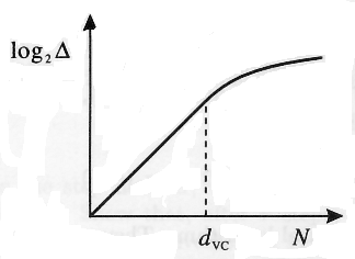
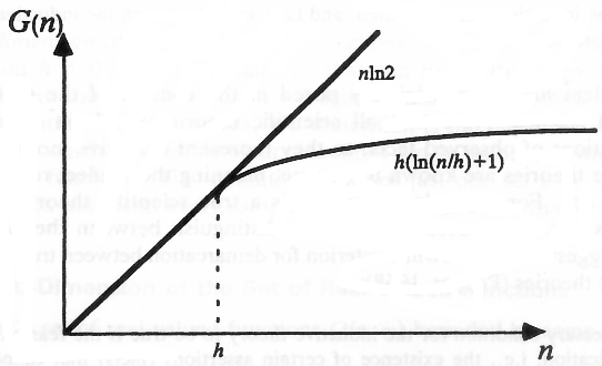
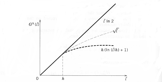
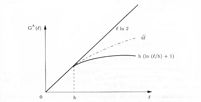
Vapnik and Chervonenkis (1968) proved that the growth function is either linear or bounded by a logarithmic function of the number of samples n (see Fig 4.2). the point n = h where the growth stats to slow down is called the VC-dimension (denoted by h). If it is finite, then the Growth Function does not grow linearly for large enough samples and, in fact, is bounded by a logarithmic function:
[…]
The VC-dimension h is a characteristic of a set of functions. Finiteness of h provides necessary and sufficient conditions for the fast rate of convergence and for distribution-independent consistency of ERM learning, in view of (4.10). On the other hand, if the bound stays linear for any n,
then the VC-dimension for the set of indicator functions is (by definition) infinite. In this case any sample of size n can be split in all 2n possible ways by the functions of a learning machine, and no valid generalization is possible, in view of the condition (4.10).
Importance of finite VC-dimension for consistency of ERM learning can be intuitively explained and related to philosophical theories of nonfalsifiability (Vapnik, 1995). […]
Cherkassky and Mulier (1998), pages 99-100
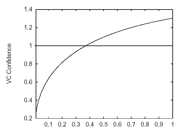
“To control the generalization ability of a learning machines one has to control two different factors: the error-rate on the training data and the capacity of the learning machine as measured by its VC-dimension. […] The two factors in (38) form a trade-off: the smaller the VC-dimension of the set of functions of the learning machine, the smaller the confidence interval, but the larger the value of the error frequency. A General way for resolving this trade-off was proposed as the principle of structural risk minimization: for the given data set one has to find a solution that minimizes their sum. A particular case of structural risk minimization principle is the Occam-Razor principle: keep the first term equal to zero and minimize the second one.”
Cortes and Vapnik (1995)
“A set of points […] for which the set […] is said to be shattered by H. If there are sets of any size which can be shattered then the growth function is equal to 2l for all l. The final ingredient in the Vapnik Chervonekis theory is an analysis of the case when there is a finite d hich is the largest size of shattered set. In this case the growth function can be bounded as follows for l > d
[…]
giving polynomial growth with exponent d. The value d is known as the Vapnik Chervonenkis (VC) dimension of the class H, denoted by VCdim(H). These quantities measure the richness or flexibility of the function class, something that is also often referred to as its capacity. Controlling the capacity of a learning system is one way of improving its generalisation accuracy. Putting the above bound on the growth function together with the observation about the fraction of permutations for which the first half of the sample is able to mislead the learner, we obtain the following bound on the left hand side of inequality (4.2):
[…]
Remark 4.2 The theorem shows that for infinite sets of hypotheses the problem of overfitting is avoidable and the measure of complexity that should be used is precisely the VC dimension. The size of training set required to ensure good generalisation scales linearly with this quantity in the case of a consistent hypothesis.
VC theory provides a distribution free bound on the generalisation of a consistent hypothesis, but more than that it can be shown that the bound is in fact tight up to log factors, as the following theorem makes clear.
[…]”
Cristianini and Shawe-Taylor (2000)
The Vapnik-Chervonenkis dimension is a way of measuring the complexity of a class of functions by assessing how wiggly its members can be.
The VC dimension of the class {f(x, α)} is defined to be the largest number of points (in some configuration) that can be shattered by members of {f(x, α)}.
A set of points is said to be shattered by a class of functions if, no matter how we we (sic) assign a binary label to each point, a member of the class can perfectly separate them.
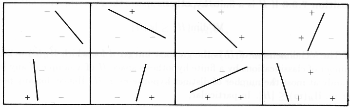
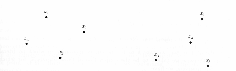
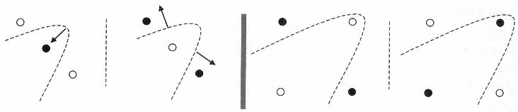
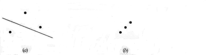
Figure 7.6 shows that the VC dimension of linear indicator functions in the plane is 3 but not 4, since no four points can be shattered by a set of lines. In general, a linear indicator function in p dimensions has VC dimension p + 1, which is also the number of free parameters. On the other hand, it can be shown that the family sin(αx) has infinite VC dimension, as Figure 7.5 suggests. By appropriate choice of α, any set of points can be shattered by this class (Exercise 7.7).
So far we have discussed the VC dimension only of indicator functions, but this can be extended to real-valued functions. The VC dimension of a class of real-valued functions {g(x, α)} is defined to be the VC dimension of the indicator class {I(g(x, α) – β > 0)}. where β takes values over the range of g.
One can use the VC dimension in constructing an estimate of in-sample prediction error; different types of results are available. Using the concept of VC dimension, one can prove results about the optimism of the training error when using a class of functions. […]
Hastie, Tibshirani and Friedman (2001)
Restriction to particular hypothesis spaces of limited size is one form of bias that has been explored to facilitate learning.41 In addition to the cardinality of the hypothesis space, a parameter known as the Vapnik-Chervonenkis (VC) dimension of the hypothesis space has been shown to be useful in quantifying the bias inherent in a restricted hypothesis space. The VC dimension of a hypothesis space H, denoted VCdim(H), is defined to be the maximum number d of instances that can be labeled as positive and negative examples in all 2d possible ways, such that each labeling is consistent with some hypothesis in H.15,55 […]” Haussler and Warmuth (1995) In: Wolpert
This result is fundamental as it shows that we can upper bound the richness NH of the hypothesis space by an integer summary—the VC dimension. A lot of research has been done to obtain tight upper bounds on the VC dimension which has, by definition, the following combinatorial interpretation: If ?H = {{(x, y) ∈ Z | l0-1(h(x), y) = 1} | h ∈ H} is the induced set of events that a hypothesis h ∈ H labels (x, y) ∈ Z incorrectly, then the VC dimension ? of ?H is the largest natural number ? such that there exists a sample z ∈ Z? of size ? which can be subdivided in all 2? different ways by (set) intersection with ?H. Then we say that ?H shatters z. If no such number exists we say that the VC dimension of ?H or H is infinite. Sometimes the VC dimension is also called the shatter coefficient
[…]
An important property of the VC dimension is that it does not necessarily coincide with the number of parameters used. This feature is the key to seeing that, by studying convergence of expected risks, we are able to overcome a problem which is known as curse of dimensionality: […]
Herbrich (2002), pages 128-130
“How do support vector machines implement structural risk minimization? Vapnik showed that there is a connection between the margin and the VC-dimension.
[…]
The lemma states that the VC-dimension is lower the larger the margin. Note that the VC-dimension of maximum-margin hyperplanes does not necessarily depend on the number of features! Instead the VC-dimension depends on the Euclidian length ? of the weight vector ? optimized by the support vector machine. Intuitively, this means that the true error of a separating maximum-margin hyperplane is close to the training error even in high-dimensional spaces, if it has a small weight vector. However, bound (2) does not directly apply to support vector machins, since the VC-dimension depends on the location of the examples [Vapnik, 1995]. The bounds in [Shawe-Taylor et al., 1996] account for this data dependency. An overview is given in [Cristianini and Shawe-Taylor, 2000].
Joachims (2002)
“Let us consider a few natural geometric concept classes, and informally calculate their VC dimension. It is important to emphasize the nature of the existential and universal quantifiers in the definition of VC dimension: in order to show that the VC dimension of a class is at least d, we must simply find some shattered set of size d. In order to show that the VC dimension is at most d, we must show that no set of size d+1 is shattered. For this reason, proving upper bounds on the VC dimension is usually considerably more difficult than proving lower bounds. The following examples are not meant to be precise proofs of the stated bounds on the VC dimension, but are simply illustrative exercises to provide some practice thinking about the VC dimension.”

Kearns and Vazirani (1994)
“The VC (Vapnik-Chervonekis) dimension h is a property of a set of approximating functions of a learning machine that is used in all important results in the statistical learning theory. Despite the fact that the VC dimension is very important, the unfortunate reality is that its analytic estimations can be used only for the simplest sets of functions. The basic concept of the VC dimension is presented first for a two-class pattern recognition case and then generalized for some sets of real approximating functions.
Let us first introduce the notion of an indicator function iF(x, w), defined as the function that can assume only two values, say iF(x, w) ∈ {-1,1}, ∀x,w. (A standard example of an indicator function is the hard limiting threshold function given as iF(x, w) = sign(xTw); see fig. 2.7 and section 3.1.) In the case of two-class classification tasks, the VC dimension of a set of indicator functions iF(x, w) is defined as the largest number h of points that can be separated (shattered) in all possible ways. For two-class pattern recognition, a set of l points can be labeled in 2lpossible ways. According to the definition of the VC dimension, given some set of indicator functions iF(x, w), if there are members of the set that are able to assign all labels correctly, the VC dimension of this set of functions h = l.
[…]
”
Kecman (2001)
”
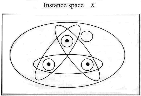
7.4.1 Shattering a Set of Instances
The VC dimension measures the complexity of the hypothesis space H, not by the number of distinct hypotheses |H|, but instead by the number of distinct instances from X that can be completely discriminated using H. To make this notion more precise, we first define the notion of shattering a set of instances. Consider some subset of instances S ⊆ X. For example, Figure 7.3 shows a subset of three instances from X. Each hypothesis H from H imposes some dichotomy on S; that is, h partitions S into the two subsets {x ∈ S|h(x) = 1} and {x ∈ S|h(x) = 0}. Given some instance set S, there are 2|S| possible dichotomies, though H may be unable to represent some of these. We say that H shatters S if every possible dichotomy of S can be represented by some hypothesis from H.
Definition: A set of instances S is shattered by hypothesis space H if and only if for every dichotomy of S there exists some hypothesis in H consistent with this dichotomy.
Figure 7.3 illustrates a set S of three instances that is shattered by the hypothesis space. Notice that each of the 23 dichotomies of these three instances is covered by some hypothesis. Note that if a set of instances is not shattered by a hypothesis spaces, then there must be some concept (dichotomy) that can be defined over the instances, but that cannot be represented by the hypothesis space. The ability of Hto shatter a set of instances is thus a measure of its capacity to represent target concepts defined over these instances.
7.4.2 The Vapnik-Chervonenkis Dimension
The ability to shatter a set of instances is closely related to the inductive bias of a hypothesis space. Recall from Chapter 2 that an unbiased hypothesis space is one capable of representing every possible concept (dichotomy) definable over the instance space X. Put briefly, an unbiased hypothesis space H is one that shatters the instance space X. What if H cannot shatter X, but can shatter some large subset Sof X? Intuitively, it seems reasonable to say that the larger the subset of X that can be shattered, the more expressive H. The VC dimension of H is precisely this measure.
Definition: The Vapnik-Chervonekis dimension, VC(H), of hypothesis space H defined over instance space X is the size of the largest finite subset of X shattered by H. If arbitrarily large finite sets of X can be shattered by H, then VC(H) ≡ ∞.
Note that for any finite H, VC(H) ≤ log2|H|. To see this, suppose that VC(H) = d. Then H will require 2d distinct hypotheses to shatter d instances. Hence, 2d ≤ |H|, and d = VC(H) ≤ log2|H|.”
Mitchell (1997)
“A simple hypothesis space (small VC-dimension) will probably not contain good approximating functions and will lead to a high training (and true) error. On the other hand a too rich hypothesis space (large VC-dimension) will lead to a small training error, but the second term in the right-hand side of (3.2) will be large. This reflects the fact that for a hypothesis space with high VC-dimension the hypothesis with low training error may just happen to fit the training data without accurately predicting new examples.”
Joachims (2002)
“The so-called VC dimension provides a measure roughly analogous to, but more general than, the ln|H measure obtained from PAC analysis. The VC dimension can be applied to continuous function classes, to which standard PAC analysis does not apply. PAC-learning theory and VC theory were first connected by the “four Germans” (none of whom actually is German): Blumer, Ehrenfeucht, Haussler, and Warmuth (1989).”
Russell and Norvig (2003)
“The VC-dimension h is a property of the hypothesis space H (written as VCdim(H) = h). It is a non-negative integer which can be infinite, and is a measure of complexity or expressive power of the family of classification functions realized by the learning machine that can be implemented using H. For many cases h is proportional to the number of free parameters of {f(·,α)}. The VC-dimension is therefore a capacity measure of the family of classification functions realized by the learning machine.
[…]
In other words, the VC dimension can be interpreted as the largest number of data points that can be separated in all possible ways by the functions contained in the space H. This is same as the maximal number of training examples that can be learned by the machine without error for all possible binary labelings of the training data. One has to be aware that it is not necessary that for a given VC dimension h, every set of h points can be shattered. This is only guaranteed for at least one case.”
Rychetsky (2001), pages 15-16
The best-known capacity concept of VC theory is the VC dimension, defined as the largest number h of points that can be separated in all possible ways using functions of the given class (cf. chapter 4). An example of a VC bound is the following: if h < l is the VC dimension of the class of functions that the learning machine can implement, then for all functions of that class, with a probability of a least 1 – ?, the bound
[…]
Schölkopf, Burges and Smola (1999)
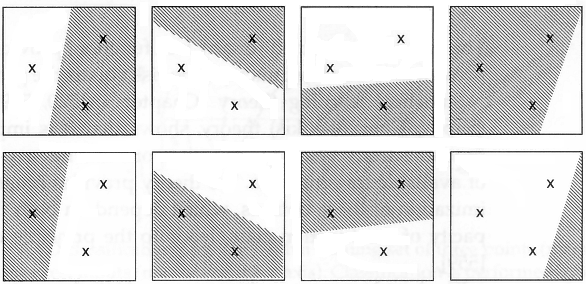
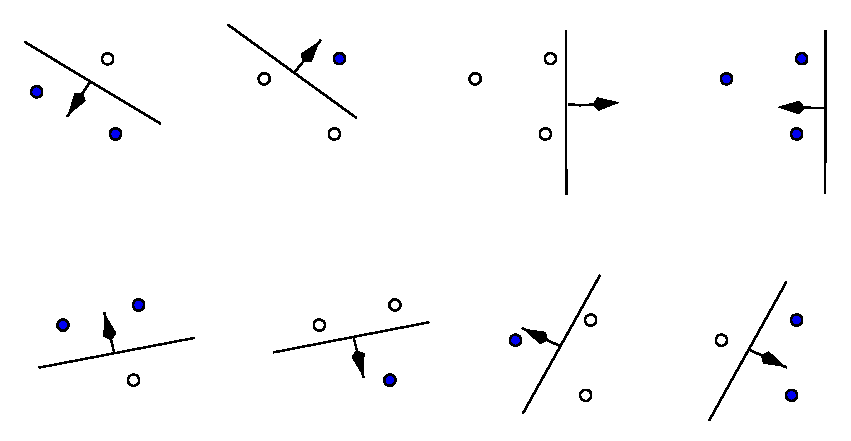
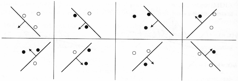
“A simple VC dimension example. There are 23 = 8 ways of assigning 3 points to two classes. For the displayed points in R2, all 8 possibilities can be realized using separating hyperplanes, in other words, the function class can shatter 3 points. This would not work if we were given 4 points, no matter how we placed them. Therefore, the VC dimension of the class of separating hyperplanes in R2 is 3.
The best-known capacity concept of VC theory is the VC dimension, defined as follows: each function of the class separates the patterns in a certain way and thus induces a certain labelling of the patterns. Since the labels are in {±1}, there are at most 2m different labellings for m patterns.”
Schölkopf and Smola (2002)
“The VC dimension h of a space of {-1,1}-valued functions, G, is the size of the largest subset of domain points that can be labelled arbitrarily by choosing functions only from G.
The VC dimension can be used to prove high probability bounds on the error of a hypothesis chosen from a class of decision functions G—this is the famous result of Vapnik and Chervonenkis [1971]. The bounds have since been improved slightly by Talagrand [1994]—see also [Alexander, 1984].
[…]
-
-
- The first drawback is that the VC dimension must actually be determined (or at least bounded) for the class of interest—and this is often not easy to do. (However, bounds on the VC dimension hhave been computed for many natural decision function classes, including parametric classes involving standard arithmetic and boolean operations. See Anthony and Bartlett [1999] for a review of these results.)
- The second (more serious) drawback is that the analysis ignores the structure of the mapping from training samples to hypotheses, and concentrates solely on the range of the learner’s possible outputs. Ignoring the details of the learning map can omit many of the factors that are crucial for determining the success of the learning algorithm in real situations.
[…]
Smola
-
et al
-
- . (2000), pages 10-11
“In this case of VC theory one may consider sets of functions with increasing VC dimension. The larger this VC dimension the smaller the training set error can become (empirical risk) but the confidence term (second term in (2.34)) will grow.”
Suykens et al. (2002)
Definition. The capacity of a set of functions with logarithmic bounded growth function can be characterized by the coefficient h. The coefficient h is called the VC dimension of a set of indicator functions. [Abbreviation for the Vapnik-Chervonekis dimension.] It characterizes the capacity of a set of functions. When the growth function is linear the VC dimension is defined to be infinite.
Below we give an equivalent definition of the VC dimension of a set of indicator functions that stress the constructive method of estimating the VC dimension.
Definition. The VC dimension of a set of indicator functions Q(z, α), α ∈ Λ, is equal to the largest number h of vecors z1, …, zl that can be separated into two different classes in all the 2h possible ways using this set of functions (i.e., the VC dimension is the maximum number of vectors that can be shattered by the set of functions).
If for any n there exists a set of n vectors that can be shattered by the functions Q(z, α), α ∈ Λ, then the VC dimension is equal to infinity.
Therefore to estimate VC dimension of the set of functons Q(z, α), α ∈ Λ, it is sufficient to point out the maximal number h of vectors […] that can be shattered by this set of functions.”
Vapnik (1998)
Definition. We will say that the VC dimension of the set of indicator functions Q(z, α), α ∈ Λ is infinite if the growth function for this set of functions is linear.
We will say that the VC dimension of the set of indicator functions Q(z, α), α ∈ Λ, is finite and equals h if the corresponding growth function is bounded by a logarithmic function with coefficient h.
[…]
…are valid, the finiteness of the VC dimension of the set of indicator functions implemented by a learning machine is a sufficient condition for consistency of the ERM method independent of the probability measure. Moreover, a finite VC dimension implies a fast rate of convergence.
Finiteness of the VC dimension is also a necessary and sufficient condition for distribution-independent consistency of ERM learning machines. The following assertion holds true (Vapnik and Chervonekis, 1974):
If uniform convergence of the frequencies to their probabilities over some set of events (set of indicator functions) is valid for any distribution function F(x), then the VC dimension of the set of functions is finite.
The VC dimension of a set of indicator functions (Vapnik and Chervonekis, 1968, 1971)
The VC dimension of a set of indicator functions Q(z, α), α ∈ Λ, is the maximum number h of vectors z1,…, zh that can be separated into two classes in all 2h possible ways using functions of the set [Any indicator function separates a given set of vectors into two subsets: the subset of vecors for which this indicator function takes the value 0 and the subset of vectors for which this indicator function takes the value 1.] (i.e., the maximum number of vectors that can be shattered by the set of functions). If for any n there exists a set of n vectors that can be shattered by the set Q(z, α), α ∈ Λ, then the VC dimension is equal to infinity.
The VC dimension of a set of real functions (Vapnik, 1979)
Let A ≤ Q(z, α) ≤ B, α ∈ Λ, be a set of real functions bounded by constants A and B (A can be -∞ and B can be ∞).
Let us consider along with the set of real functions Q(z, α), α ∈ Λ, the set of indicators (Fig. 3.1)
-
- where
θ
-
- (
z
-
- ) is the step function
θ
-
- (
z
-
- ) = 0 if
z
-
- < 0, 1 if
z
-
- ≥ 0.
-
- The
VC dimension of a set of real functions
Q
-
- (
z
-
- , α), α ∈ Λ, is defined to be the VC dimension of the set of corresponding indicators (3.22) with parameters α ∈ Λ and β ∈ (
A
-
- ,
B
-
- ).
-
- Vapnik (2000), pages 79-80
c “costs” or “generalization errors”
d “training set”
ε
f “target” input-output relationships
H hypothes class
h hypotheses
m number of elements in the training set
s training set error
“The VC framework is in many ways similar to both the SP framework and PAC. All three are conventionally defined in terms of iid likelihood and iid error. They also all have mrather than d fixed in their distribution of interest (unlike the Bayesian framework), and all can be cast with f fixed in that distribution.
Cast in this f-fixed form, the (vanilla) VC framework investigates the dependence of the confidence interval P(|c – s| > ε|f, m) on m, s, the learning algorithm, and potentially f(recall that s is the empirical misclassification rate), Sometimes the value of P(|c – s|≤ ε|f, m) for one particular set of values for c, s, f, and m is called one’s “confidence” that |c – s| ≤ ε. Note that if one has a bound on P(|c – s| > ε|f, m), then one also has a bound on P(c > s + ε|f, m). Some researchers interpret this—incorrectly, as is demonstrated below—to be bound on how poor c can be for a particular observed s. (Such misinterpretations are a direct result of the widespread presence in the VC literature of the first sin discussed in the introduction.)
The famous “VC dimension” is a characterization of H~, the h-space support of a learning algorithm P(h|d). For current purposes (i.e., Y = {0, 1} and our error function), it is given by the smallest m such that for any dX of size m, all of whose elements are distinct, there is a dY for which no h in H~ goes through d. (The VC dimension is the smallest number minus one.) It turns out that in a number of scenarios, as far as P(|c – s| > ε|f, m) is concerned, what is important concerning one’s algorithm is its VC dimension. In particular, one major result of the VC dimension of the learning algorithm. (Accordingly, the challenge in the VC framework is usually to ascertain the VC dimension of one’s generalizer.)
[…]
-
-
- The VC framework is concerned with confidence intervals P(|c – s| > ε|f, m) for variable ε.
- The VC dimension is a characterization of the support (over all h’s) of P(h|d). Many theorems bounding P(|c – s| > ε|f, m) depend only on m, the VC dimension of the generalizer, and ε. In particular, such results hold for all f and/or P(f) and for any generalizer of the given VC dimension.
- In the illustrative case where P(h|d) always guesses the same h, c does not vary in P(|c – s| > ε|f, m); rather s does. (s is determined by the random variable dX, which is unspecified in the conditioning event.) In all the other frameworks c varies.
- This motivates the analogy of viewing the VC framework as coin-tossing; one has a coin of bias-towards-heads c, and flips it m times. The VC frameworks’ distribution of interest is analogous to the coin-flipping distribution P(|c – s| > ε|c, m). This coin-flipping distribution concerns the probability that the empirically observed frequency of heads will defer much from s. This probability does not directly address the process of observing the empirical frequency of heads and then seeing if the bias-towards-heads differs much from that observed frequency. That process instead concerns P(|c – s| > ε|s, m).
- Accordingly VC results do not directly apply to distributions like P(c|s, m); one can not use VC results to bound the probability of large error based on an observed value of s and the VC dimension of one’s generalizer. Note no recourse to off-training-set error is needed for this result.
- The behavior of P(|c – s| > ε|f, m) for off-training-set error is not currently well understood.”
-
Wolpert In: Wolpert (1995), pages 165-166, 173-174
Leave a Reply
You must be logged in to post a comment.